big_vision
is an open-source research codebase created and maintained by
Alexander Kolesnikov, Xiaohua Zhai,
and myself during our time at Google Brain and DeepMind1,
with major core contributions by Andreas Steiner and André Susano Pinto.
It is widely used internally, including for key research such as ViT, SigLIP, and PaliGemma.
The codebase's philosophy is to remain simple and compact even as it grows,
such that an individual familiar with JAX
can read and understand it fully within one good afternoon.
However, it is criminally under-documented, and mainly used on Google internal and Cloud TPUs.
With this article, I aim to slightly alleviate this issue by walking through a few examples of typical single-machine GPU use-cases.
This is not an official Google documentation, but my personal journey.
Fine-tuning PaliGemma, SigLIP, and training ResNet
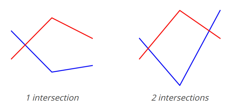
We'll use the "count line intersections" task from the VLMs are blind paper, because it's simple to create data and I was curious about it anyways.
We'll do three things here:
- First, we'll fine-tune PaliGemma on this data, VQA-style.
- Then, noticing this is a classification problem, we'll fine-tune the SigLIP vision encoder as a good-old classifier.
- Finally, we'll train a small ResNet classifier from scratch, as a baseline.
- Here, we'll also look into augmentations.
- We'll also cover how to run single-machine (but multi-GPU) sweeps.
I won't do much tuning or result analysis here, as this meant to focus on explaining big_vision.
I'll discuss the task itself, and more results, in a separate future article.
But since I know you're curious, and I have the numbers for 128 training examples:
| No Augs | With Augs | |
|---|---|---|
| PaliGemma-3B (pretrained) | 95.9% | 97.8% |
| SigLIP-So400m (pretrained) | 96.6% | 98.7% |
| BiT ResNet-26 (from scratch) | 52.9% | 93.6% |
(Those are results on test with best hparams selected on val, i.e. everything's proper.)
Installation
We generally have two options:
- You have a dedicated machine that you're using almost all the time.
In this case, install
big_visionin a virtualenv once and then use it from there. - You use a cloud-based GPU provider like RunPod, Lambda Labs, vast.ai, Lightning.ai, or others. In this case, you typically spin machines up and down as needed, sometimes with a single small GPU, sometimes with 8 large GPUs. Then, you typically prepare a Docker image with everything installed, so the machine is set-up and ready to go once spun up.
Manual installation
Just start a machine on your favourite provider with a working CUDA. For this project, we'll need at least 32GB of total GPU memory, so a single A40 hits this pretty well and is very cheap (on RunPod currently $0.39/h). Two 16GB GPUs would work too, completely transparently. We could get away with less if I spent time tuning the config more, but here I'll do full fine-tuning, becasue it's already pretty cheap anyways!
SSH into it and let's get started (on RunPod, do unminimize first) with a virtualenv:
python -m venv venv
. venv/bin/activate
pip install -U pip
pip install -U "jax[cuda12]"  # Not gonna age well.

git clone https://github.com/lucasb-eyer/big_vision.git
pip install -r big_vision/big_vision/requirements.txt
I'm using my fork as I currently have a few small fixes there. And now let's download the PaliGemma base model weights. Sadly, for this we need to ACK some license either on HF or Kaggle, and only then can download them:
pip install -U "huggingface_hub[cli]"
huggingface-cli login
huggingface-cli download google/paligemma-3b-pt-224-jax paligemma-3b-pt-224.npz --local-dir /workspace
mv /workspace/{paligemma-3b-pt-224,pt_224}.npz  # Need to rename it...
And we're ready to start training! Well, almost, need the dataset and config next...
Docker image
The best way to create a docker image is to use some starting template from the GPU provider you'll be using where you verified the GPU/CUDA works, and then add more layers on top.
I initially felt most comfortable with RunPod, so I decided to create RunPod docker images / templates for JAX+big_vision on RunPod, but the process should be similar everywhere.
It's really just a docker-ization of the above manual install commands, and a little bit of trickery to avoid storing secrets like HF_TOKEN in the image. I won't write a full Docker tutorial here or repeat the whole file, but I did put the Dockerfile in the accompanying repo if you're interested or need a starting point.
In case you're using RunPod, I created templates with these dockerfiles that you can just use:
- JAX +
big_visionon CUDA12 - JAX +
big_visionon CUDA12 with PaliGemma base 224px checkpoint baked in - JAX +
big_visionon CUDA12 with PaliGemma base 448px checkpoint baked in - JAX +
big_visionon CUDA12 with PaliGemma base 896px checkpoint baked in
Or just search for big_vision when starting a new pod.
Preparing the dataset
Overview
There are three components to data: the data source, the data input pipeline, and the data preprocessing.
For the input pipeline, which is the part of the code getting the data from its source into mini-batches, big_vision relies entirely on tf.data.
While annoyingly tied to TensorFlow, this is still the only publicly available, scalable and efficient input pipeline in town.
Although alternatives are being developed (grain, datago, webdataset pipeline, mosaic streaming, ...), they were not fully there yet.
The data preprocessing includes things such as image resizing, text formatting, and random augmentations.
We developed our own mini-language for registering and composing arbitrary processing steps that has worked really well for many years,
which we call pp (short for pre-processing)
throughout the codebase, and currently mostly uses TensorFlow ops,
although that is slowly changing.
The data source is the on-disk format of the dataset itself, including the ways in which it can be sliced and diced.
big_vision historically relies on TensorFlow Datasets (TFDS) which, despite the name, is distancing itself from TensorFlow.
The main advantage is that it has a very solid and deterministic slicing and dicing API.
However, we also created a JSON-L data source,
as that format is a lot simpler to work with and good enough for small/mid dataset sizes.
Creating the JSON-L dataset
The JSON-L format is very simple: one json object per line. The values in the json object can be:
- Plain values such as integers, lists, or strings.
- Filenames, which are then loaded from disk.
- URLs, which are then loaded from the web and cached locally.
The latter two are usually used for image and audio data.
We'll give our line-intersection dataset the following structure:
{"image": "/path/to/image.file", "label": 0}
This works for classification, and we'll use pp ops to turn it into a prompt and answer strings for the VLM.
Simply write a file with one line per example, and you have a dataset.
I developed the data generation code in a Jupyter Notebook, and once done and verified, copy-pasted it into a quick'n'dirty python script that generates both the images and the jsonl file. The salient part for the jsonl creation is this loop:
rng = np.random.default_rng(1337)
with open('lines_data/train.jsonl', 'w+') as f:
  for fname in (f'train_{i:05d}.png' for i in tqdm(range(10_000))):
    img, c = generate(rng=rng)
    cv2.imwrite('lines_data/' + fname, img)
    f.write(json.dumps({'label': c, 'image': fname}) + "\n")
That's it. We'll get to the pre-processing when we write the config file for the fine-tuning job.
To generate the data, run that script.
I'm using uv to handle deps, so install uv first, then run it:
curl -LsSf https://astral.sh/uv/install.sh | sh
cd /workspace
uv run make_lines.py  # Creates them in a subfolder
High-level codebase structure
The main audience for the codebase is our own research team, and this is important to understand the structure.
Generally, we wanted different projects to be somewhat separated, but also benefit from each other and thus not completely separate.
That's why the codebase has a "transposed" layout: there are top-level folders for the usual suspects: models, pre-processing ops (pp), configs, trainers, ...
However, inside each we have three layers: core, projects, and xp (experimental).
The core files are right there and contain only things that are useful across many projects, for example the vit.py model.
Individual proejcts are in proj/PROJECT_NAME subfolders, but may also import things from other projects.
Finally, xp/THING is the place for very experimental code that is usually never published.
This unorthodox structure has allowed the codebase to flourish while remaining largely coherent over more than five years and with many different teams, without slowing us down.
For reading the code, a good entry point is the trainer of the project you're interested in.
That should mostly be readable and skimmable. Then, a project's config file defines all kinds of details about the training,
and usually contains extra info on how to run it.
PaliGemma fine-tuning
For fine-tuning the full VLM, we will slightly reformulate the task as a language task, even though it's a bit of an abuse of formulation.
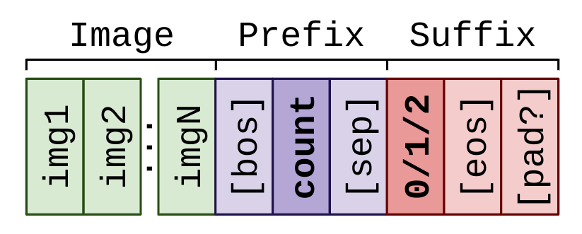
PaliGemma (and, really, all VLMs) takes as input an image and a prefix, which is a textual input (usually a question or a command), and produces a suffix, which is a textural output (the answer).
To make the abuse of formulation absolutely obvious, I'll keep the language "brief and concise", and decide for the following format:
image: 224x224 pixels. The smallest resolution is enough for this task; I generated the images in that resolution in the first place.prefix: Since the question is always the same and doesn't really contain any user input, I'll go for a single word that's somewhat relevant to the task:count. The<BOS>and<SEP>tokens are automatically added by PaliGemma'scombine_and_keep_{train,eval}utility functions that we'll use.suffix: The only possible answers are 0/1/2. I'll keep it simple again and use these numbers as the only answer token.
Thus, overall, the data we're preparing and will be input to the model looks as follows:
Writing the PaliGemma config file
The config file's get_config function is executed by the trainer and should return the full
ConfigDict
(a nested dictionary with .-access syntax, kinda JS-like) with all fine-tuning settings.
There is no full reference of configs, as what is available depends on the trainer, model, ... used,
it's best to read the trainer code and look at other/similar configs.
For PaliGemma, we prepared a fork_me.py
config file that is heavily commented and should be used as starting point for a new PaliGemma fine-tuning.
But because I like to fiddle with stuff, I further simplified it for this post. Here we go:
First, the entry function which creates the config:
def get_config(arg=None):
  # You probably do NOT want to add settings here. The `arg` way of settings is
  # really only for things you'd want to sweep and which affect MULTIPLE config
  # settings at once or go into the pp string.
  c = bvcc.parse_arg(arg, freeze_vit=False, freeze_llm=False)
This initializes the ConfigDict c that will be returned, and wires the arg mechanism
that can be used to parametrize complex configurations that touch multiple fields.
You can ignore this for now, we'll get back to it later.
  c.input = training_data()

  # And elsewhere:
def training_data():
  """Creates training data config."""
  c = bvcc.parse_arg('')  # Just make a configdict without extra import.
  c.data = dict(
    name='bv:jsonl',
    fname='/workspace/lines_data/train.jsonl',
    # The strings in the `image` key of the JSON-L are files in that folder:
    fopen_keys={'image': '/workspace/lines_data/'},
    # Or they could be URLs to download:
    # download_keys=['image'],
    stop=128,  # Only use 128 examples. float("inf") for all.
  )
  c.pp = '|'.join([
    # Even though the images are already 224, we'll still reshape them
    # in order to give the variable a static shape.
    'decode|resize(224)|value_range(-1, 1)',
    'strfmt("count", outkey="prefix")',  # Store string "count" in `prefix`
    'strfmt("{label}", outkey="suffix")',  # Format label as string in `suffix`
    combine_and_keep_train(text_len=8),  # Combine prefix+suffix to 8 toks.
  ])
  # Keep the whole dataset in RAM after first pass. Useful optimization for
  # small/mid-size datasets, but risks a host OOM for large datasets.
  c.cache_raw = True
  return c
This defines the training data: c.data describes the data source
(our JSON-L file, note we only train on the first 128 examples)
whereas c.pp is the data pre-processing definition.
In a nutshell, the pre-processing works as follows: a "data dictionary", such as a single line of the JSON-L file, gets passed through a sequence of processing functions ("pp ops"), at the end of which it has become one example of the minibatch.
This sequence of pp ops is defined by a string mini-language.
Each op is defined somewhere in a file in the pp/ folder,
for example strfmt is defined here.
The op returns a function which takes in an example (dict), and returns a new (processed) example (dict).
Thus, the pre-processing string we defined here can be understood as follows:
'decode|resize(224)|value_range(-1, 1)',
This first decodes the raw (png, jpg, ...) image into an array of rgb values.
Then, it resizes that image to a fixed 224x224 resolution.
Finally, it rescales the pixel values from the original [0, 225] range into the range [-1, 1].
That's it for the image, next:
    'strfmt("count", outkey="prefix")',  # Store string "count" in `prefix`
    'strfmt("{label}", outkey="suffix")',  # Format label as string in `suffix`
These create two strings: The key prefix simply is the fixed string "count",
whereas the key suffix is our label key's content turned into a string.
At this point, the content of an example has been processed to look somewhat like this, if the image has two intersections:
{"prefix": "count", "suffix": "2", "image": [float32 array of shape 224,224,3]}
Finally, we have a PaliGemma-specific utility function that defines a somewhat cumbersome
sequence of preprocessing ops that tokenize the prefix and suffix, combine them with a separator,
either pads or truncates, resulting in a single tokenized text field along with a
mask_ar indicating the auto-regressive part of text, and mask_loss indicating where in
text a training loss should be applied (usually they are the same):
combine_and_keep_train(text_len=8), # Combine prefix+suffix to 8 toks.
It also removes no longer needed keys. So after this, our example looks as follows:
{
  "image": [float32 array of shape 224,224,3],
  "text": [2, 1656, 108, 235284, 1, 0, 0, 0],
  "mask_ar": [0, 0, 0, 1, 1, 1, 1, 1],
  "mask_loss": [0, 0, 0, 1, 1, 0, 0, 0],
}
Oh, and the c.cache_raw = True is a useful optimization for small datasets without,
augmentations; it means to keep the complete data after decoding and processing in
CPU cache (RAM), so the second epoch and beyond will be faster.
Now back to the main get_config meat:
  # Instead of epochs, you can also use `total_examples` or `total_steps`.
  c.total_epochs = 15
  c.input.batch_size = 32
  c.optax_name = 'big_vision.scale_by_adafactor'
  c.lr = 1e-5
  c.wd = 3e-7
  c.grad_clip_norm = 1.0
  c.label_smoothing = 0.0
These were just a bunch are relatively mundane and self-describing settings.
Worth noting is that everything related to time/duration can be expressed in terms
of steps, epochs, examples, or percent; so while we specify the training
duration as total_epochs, we could also have used total_steps or total_examples
instead, whichever is most convenient for the situation.
Continuing:
  # Learning-rate schedule. Probably is fine like this.
  sched = dict(decay_type='cosine', warmup_percent=0.05)
  c.schedule = [
      ('img/.*', None if c.freeze_vit else sched),
      ('llm/.*', None if c.freeze_llm else sched),
  ]
This defines the schedule, which affects both learning-rate and weight-decay.
We can apply different schedules to different parts of the model,
and applying a None schedule to a parameter means to freeze it.
For each model parameter, the list of (regex, schedule) pairs is processed
from top to bottom, and the first regex that matches defines the schedule
for that parameter. We have safeguards for missing parameters, check the logs.
A shortcut for the simple case of applying the same schedule to all parameters
is simply c.schedule = dict(decay_type='cosine', warmup_percent=0.05).
We have the same mechanism to allow applying learning-rate or weight-decay multipliers
to different parts of the model, called lr_mult and wd_mult, for example:
c.lr_mult = [('img/.*', 0.1), ('.*', 1.0)]
would apply a 10x smaller learning-rate to the image encoder than to everything else. OK, moving on:
  # Model section.
  c.model_name = 'proj.paligemma.paligemma'
  c.model = {}
  c.model.img = dict(variant='So400m/14', pool_type='none', scan=True)
  c.model.llm = dict(vocab_size=256_000 + 1024 + 128, dropout=0.0)
  c.model_init = 'pt_224'
This defines the model, and should mostly be unchaged for PaliGemma.
The model_init describes which checkpoint to load.
You can use a "vanity name" (each model can define its own, PaliGemma's are defined here)
as we do here, or just a file path.
Here is also where you could try setting dropout=0.1 which sometimes helps.
  # FSDP strategy.
  c.mesh = [('data', -1)]
  c.sharding_strategy = [('.*', 'fsdp(axis="data")')]
  c.sharding_rules = [('act_batch', ('data',))]
This is a very powerful and flexible configuration defining how to shard the model.
It covers basically all kinds of parallelisms, and explaining it here is beyond the scope of this article.
In short, these settings do FSDP, by defining a 1D mesh over all devices,
and sharding all parameters (.*) according to the fsdp(axis="data") strategy over them.
However, the strategy has a bit of logic
to avoid sharding tiny params.
  c.input.shuffle_buffer_size = 1000
  c.log_training_steps = 1
  c.pp_modules = ['ops_general', 'ops_image', 'ops_text', 'proj.paligemma.ops']

  c.seed = 0

  c.evals = {}
  add_eval_pplx(c)
  # add_eval_store(c)
  add_eval_acc(c)

  return c
A few more misc settings. The shuffle buffer should be larger for larger datasets,
log_training_steps is how often we log training loss. For any longer training runs
we usually just set it to 50, and for very short runs (like here), to 1 or 2.
pp_modules tells which preprocessing modules (from pp/ folder) to load.
Finally, we call a few functions that add "evaluators" to the config.
Evaluators are pieces of code in the evaluators/
folder that run at specific intervals during training and
are meant to run some evaluations or logs something interesting.
Common examples are linear probes, perplexity, VQA-decoding, ... I'll only show one here:
def add_eval_acc(c, **kw):
  """Add eval configs."""
  c.evals['eval/acc'] = dict(
First thing to note here already, is that the key name eval/acc will also be
used as prefix to any metrics that this evaluator logs.
type='proj.paligemma.transfers.vqa',
This tells us which piece of code this evaluator runs, in this case it is
evaluators/proj/paligemma/transfers/vqa.py.
pred='decode', pred_kw={'max_decode_len': 8},
This part is non-trivial, and allows us to mix and match evaluators across projects.
An evaluator often asks for a "predict function", which runs the model the way the evaluator needs.
For example, a linear probe evaluator would need to perform just a forward pass up to the thing that's being probed.
A VQA evaluator of a VLM instead needs a function that runs a proper decoding loop which involves multiple forward passes.
How these are done depends on what training we're running.
Hence, the trainer provides a list of "predict_fn's"
that it implements, and here in the config we're telling big_vision which of our trainer's predict_fn's
is the one that this evaluator should be using. In this case, this one.
The predict_fn may take keyword arguments,
for instance our decode one can be setup to use a sampler other than greedy, and return the best_of_n decoding.
    outfile='{workdir}/vqa_eval_{step}.json',
    data=dict(
      name='bv:jsonl',
      fname='/workspace/lines_data/val.jsonl',
      fopen_keys={'image': '/workspace/lines_data/'},
    ),
    log_percent=1/8, skip_first=True, tokenizer=TOKENIZER,
    pp_fn='|'.join([
      'decode|resize(224)|value_range(-1, 1)',
      'strfmt("count", outkey="prefix")',
      'strfmt("{label}", outkey="answer")',  # GT evaluator compares to.
      'copy(inkey="id", outkey="question_id")',  # Required by evaluator.
      combine_and_keep_eval(text_len=8, keep=('answer', 'question_id')),
    ])
  )
  c.evals['eval/acc'].update(kw)
The rest was relatively mundane, setting up the evaluation frequency, this time in
log_percent so we run a total of 9 evals (one every 1/8th of training, the final one, but not the first one).
The data is defined in a similar way as for training, and we again have a pp string.
The pp ops are slightly different, to give the evaluator what it needs.
The full config file is available in the accompanying repo.
Running the PaliGemma fine-tuning
And now we can run the config file. For running big_vision, we need to be in
the same folder as big_vision's README file.
Then, we need a few environment variables set, I like to set them in the commandline, but you do you:
env XLA_PYTHON_CLIENT_ALLOCATOR=platform \
    XLA_PYTHON_CLIENT_MEM_FRACTION=.99 \
    BV_GEMMA_DIR=/workspace/ \
  python -m big_vision.trainers.proj.paligemma.train \
    --config /workspace/lba_bv_tuto/lines_paligemma.py \
    --workdir /workspace/workdir_`date '+%m-%d_%H%M'`
Note that this was all one single big-ass command-line.
The first two environment variables currently result in better-behaved GPU memory usage of JAX, see the JAX GPU memory guide for more info.
BV_GEMMA_DIR just lets big_vision know where you stored the PaliGemma checkpoint.
Then comes the actual thing that's run: python -m big_vision.trainers.proj.paligemma.train, which is the training script of big_vision's PaliGemma project.
Trainers need at the very least two arguments:
the --config file which we just wrote and defines what exactly is trained, and
the --workdir which is where logs, metrics, and checkpoints are written to.
When the workdir already contains a checkpoint, the trainer attempts to resume from it. That's why for every new run I like to automatically include the date-time in the workdir name.
There's a lot of logs especially during initialization that are useful for debugging,
but the most important progress updates are marked with a yellow [NOTE],
and training step logs with a pink [2] with 2 being the step number.
Thus, a good training that works should look something like this:
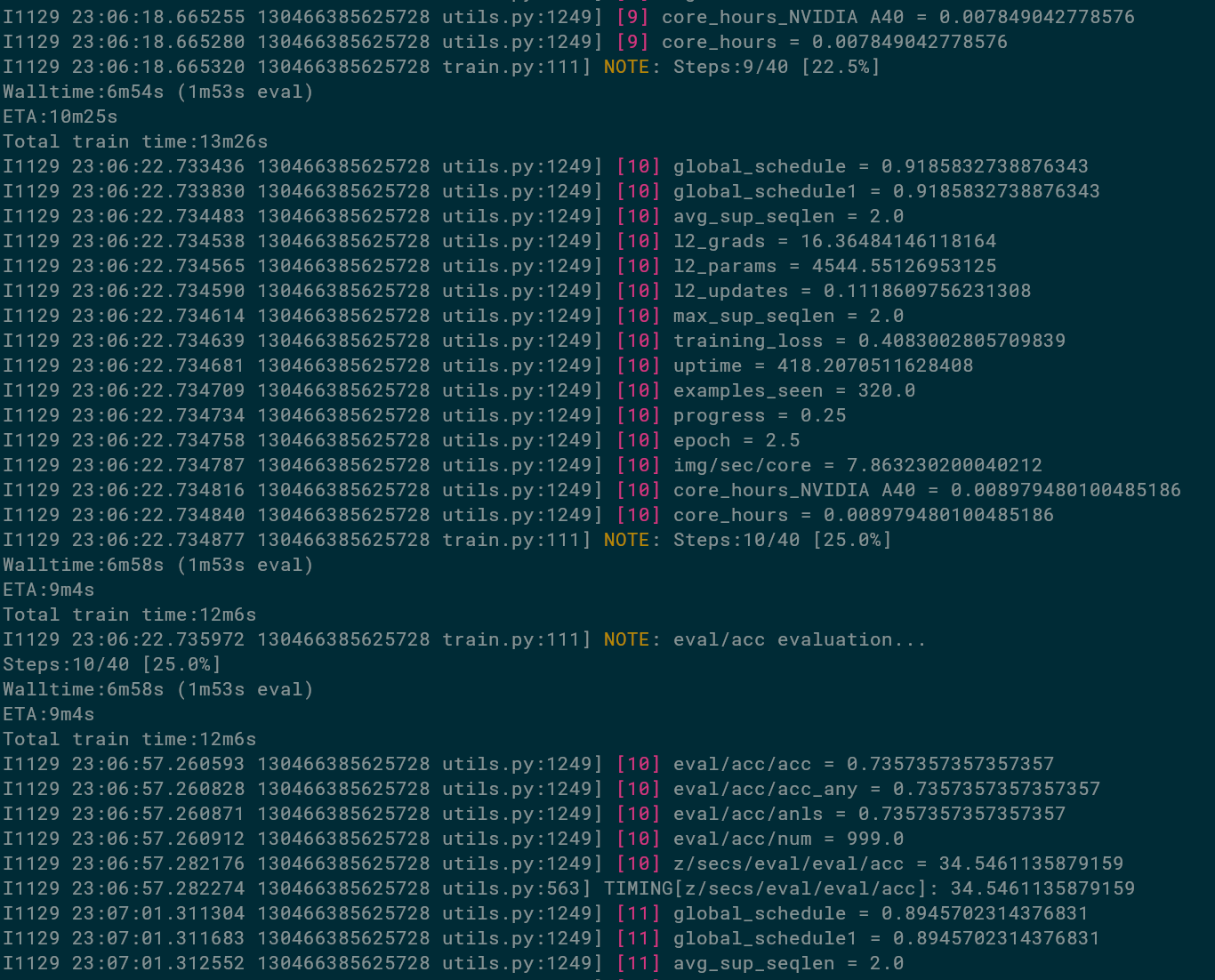
We can see that the total training time is estimated to take 12m6s,
we're already 6m58s into the training, and there's an estiamted 9m4s remaining.
We can also see that these don't add up. They are estimates from different signals,
are off in the first dozens of steps, plus wall-time includes init time.
But suffice to say, this fine-tuning is fast!
We could make it even faster by evaluating less frequently: 1m35 out of 6 was spent in evals.
We can also see that at 25% of the training, we decided to run the evaluator called eval/acc,
and it logged metrics such as eval/acc/acc being 73.6% already, evaluation being done on eval/acc/num=999 examples, and one evaluation having take 34.5 seconds.
Changing parameters
When the training is over, we see in the logs of the final eval/acc that we reached about 92.6%.
The learning-rate was not quite optimal (just trust me), so let's run again with slightly higher learning-rate.
Instead of constantly editing the config file, we can also override any config parameter on the commandline, by passing it as argument with dot-syntax:
env XLA_PYTHON_CLIENT_ALLOCATOR=platform \
    XLA_PYTHON_CLIENT_MEM_FRACTION=.99 \
    BV_GEMMA_DIR=/workspace/ \
  python -m big_vision.trainers.proj.paligemma.train \
    --config /workspace/lba_bv_tuto/lines_paligemma.py \
    --workdir /workspace/workdir_`date '+%m-%d_%H%M'` \
    --config.lr 3e-5  # <-- This right here.
Yay, now up to 94.3%! Goes to show that learning-rate is one of the most important hyper-parameters to tune. Let me remind you of the following advice we gave in our report, which is distilled from tuning many dozens of PaliGemma transfers to all kinds of tasks:
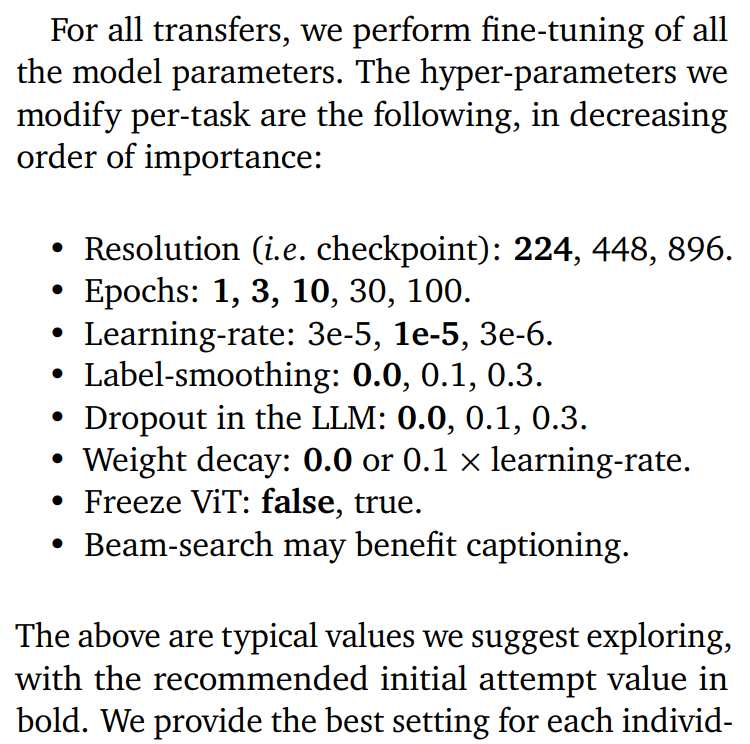
I'll show how to more systematically sweep them at the end of the article.
Looking at the results
Above we already looked at the logs and manually read the final eval scores. Of course that's not really enough to analyze runs, let's now plot curves and look at actual predictions.
Plotting some curves
Internally, we have fancy logging and plotting tools.
big_vision logs aggregate step metrics once a step, and in the open-source code we simply log these step metrics in a JSON-L file,
one step per line, in the $WORKDIR/big_vision_metrics.txt file, here's an excerpt:
{"step": 38, "global_schedule": 0.015299856662750244, "global_schedule1": 0.015299856662750244, "avg_sup_seqlen": 2.0, "l2_grads": 0.0051719495095312595, "l2_params": 4544.5390625, "l2_updates": 0.005137327592819929, "max_sup_seqlen": 2.0, "training_loss": 3.7420857552206144e-05, "uptime": 971.1271621850319, "examples_seen": 1216.0, "progress": 0.95, "epoch": 9.5, "img/sec/core": 7.345379911072726, "core_hours_NVIDIA A40": 0.04226647665504262, "core_hours": 0.04226647665504262}
{"step": 39, "global_schedule": 0.006819337606430054, "global_schedule1": 0.006819337606430054, "avg_sup_seqlen": 2.0, "l2_grads": 0.005499803926795721, "l2_params": 4544.5390625, "l2_updates": 0.002123815705999732, "max_sup_seqlen": 2.0, "training_loss": 3.810248745139688e-05, "uptime": 975.4800174080301, "examples_seen": 1248.0, "progress": 0.975, "epoch": 9.75, "img/sec/core": 7.351496514501312, "core_hours_NVIDIA A40": 0.04347560310587546, "core_hours": 0.04347560310587546}
{"step": 40, "global_schedule": 0.0017077624797821045, "global_schedule1": 0.0017077624797821045, "avg_sup_seqlen": 2.0, "l2_grads": 0.005480646621435881, "l2_params": 4544.5390625, "l2_updates": 0.0005104840965941548, "max_sup_seqlen": 2.0, "training_loss": 3.162116263411008e-05, "uptime": 979.8389665030409, "examples_seen": 1280.0, "progress": 1.0, "epoch": 10.0, "img/sec/core": 7.341219019195962, "core_hours_NVIDIA A40": 0.044686422298934006, "core_hours": 0.044686422298934006, "eval/acc/acc": 0.9429429429429429, "eval/acc/acc_any": 0.9429429429429429, "eval/acc/anls": 0.9429429429429429, "eval/acc/num": 999.0, "z/secs/eval/eval/acc": 34.36034384602681, "val/pplx/avg": 58.918144707207205, "val/pplx/sum": 412.4269894894895, "z/secs/eval/val/pplx": 32.01938859303482}
You can see here that some steps contain more metrics than others. Those are the steps where evaluation was ran, and evaluation is folded into them. This format is extremely easy and flexible to read and plot in colab with very little code:
import json

with open('metrics_lr3e-5.txt') as f:  # I renamed the file
  metrics = [json.loads(line) for line in f]

all_keys = sorted(set([k for m in metrics for k in m]))
print(f"All available keys:\n - {'\n - '.join(all_keys)}")
That's all it takes to load all the measurements in a structured way! The output prints the following, giving you an idea of what we track by default:
All available keys:
 - avg_sup_seqlen
 - core_hours
 - core_hours_NVIDIA A40
 - epoch
 - eval/acc/acc
 - eval/acc/acc_any
 - eval/acc/anls
 - eval/acc/num
 - examples_seen
 - global_schedule
 - global_schedule1
 - img/sec/core
 - l2_grads
 - l2_params
 - l2_updates
 - max_sup_seqlen
 - progress
 - step
 - training_loss
 - uptime
 - val/pplx/avg
 - val/pplx/sum
 - z/secs/eval/eval/acc
 - z/secs/eval/val/pplx
 - z/secs/update0
Let's define one tiny helper function that I like to use a lot, it extracts corresponding x and y values as numpy arrays:
import numpy as np

def xy(ms, x, y, ymul=1):
  xs = np.array([m[x] for m in ms if x in m and y in m])
  ys = np.array([m[y] for m in ms if x in m and y in m]) * ymul
  return xs, ys

with np.printoptions(precision=3, suppress=True):
  x, y = xy(metrics, 'step', 'eval/acc/acc')
  print(x, '\n', y)
  x, y = xy(metrics, 'epoch', 'training_loss')
  print(x, '\n', y)
See how we can mix-and-match arbitrary keys for x and y, and how different metrics are written at different frequencies:
[ 5 10 15 20 25 30 35 40 40]
 [0.376 0.719 0.897 0.785 0.932 0.944 0.942 0.943 0.943]
[ 0.25  0.5   0.75  1.    1.25  1.5   1.75  2.    2.25  2.5   2.75  3.
  3.25  3.5   3.75  4.    4.25  4.5   4.75  5.    5.25  5.5   5.75  6.
  6.25  6.5   6.75  7.    7.25  7.5   7.75  8.    8.25  8.5   8.75  9.
  9.25  9.5   9.75 10.   10.  ]
 [5.726 5.484 1.439 0.704 0.849 0.483 0.602 0.53  0.502 0.404 0.416 0.236
 0.714 0.511 0.274 0.247 0.169 0.287 0.048 0.047 0.074 0.103 0.297 0.003
 0.002 0.001 0.    0.002 0.001 0.    0.    0.    0.    0.    0.    0.
 0.    0.    0.    0.    0.   ]
Alright, so now let's plot a few of those:
%config InlineBackend.figure_format = 'retina'
import matplotlib as mpl

fig, axes = mpl.pyplot.subplots(1, 3, figsize=(10, 3), constrained_layout=True)
l1, = axes[0].plot(*xy(metrics, 'epoch', 'training_loss'), label='Training loss')
axes[0].set_xlabel('epoch')  # We should do log-y, but this is prettier :)
ax0twin = axes[0].twinx()
l2, = ax0twin.plot(*xy(metrics, 'epoch', 'eval/acc/acc'), c='C1', label='Val accuracy')
ax0twin.set_ylim(0, 1)
ax0twin.legend([l1, l2], [l1.get_label(), l2.get_label()], loc='center right')

axes[1].plot(*xy(metrics, 'step', 'img/sec/core'))
axes[1].set_ylim(0, None)
axes[1].set_ylabel('img/sec/core')
axes[1].set_xlabel('step')

for k in filter(lambda k: k.startswith('z/secs'), all_keys):
    axes[2].plot(*xy(metrics, 'step', k), 'o-', label=k.replace('z/secs/', ''))
axes[2].legend()
axes[2].set_ylabel('Duration [seconds]')
fig.savefig('plot.svg')

Very informative; what can we see?
- Accuracy goes up as training loss goes down, getting close to 0 as accuracy gets close to stalling. This is pretty common in fine-tuning on few examples, and one reason not to worry about over-fitting too much.
- We're getting between 7 and 8 images per second per GPU ("core" is a leftover from early TPU times). Given we pay $0.39 per GPU-hour, that gives us about 70k examples per US-dollar. That's pretty reasonable for small and mid scale fine-tuning, but 1 billion examples would cost $14k.
- Accuracy evaluation, which involves decoding from the VLM, takes about 35s per eval, except the first time it took about 48s. That's because the first time things are compiled, and for some evaluators, data might get cached or precomputed. Thus, the init time was about 13s.
- Perplexity evaluation is faster (32s) since there's no decoding, just a forward pass. However, the fact it's pretty close to accuracy evaluation tells us the decoded string in the accuracy evaluation is not very long, which indeed is true.
update0is also interesting, it's the time taken for the first training step. Again, this includes compilation of the training code (forward, backward, optim) as well as one execution of it.
I usually spend a little more time and write a few more plotting utilities to plot more things and also make them a bit prettier just because; but we'll postpone that this time.
Looking at val predictions
Since we passed a outfile='{workdir}/vqa_eval_{step}.json' argument to the VQA evaluator,
it also writes all predictions it makes to the JSON output file so we can look at them
(or upload them to an eval server).
Unfortunately there is currently a bug making the {step} parameter stuck to 0,
so we only get a single file that's constantly overwritten,
and after training we have the final predictions.
There's really not much big_vision specific here, it's jsut a json file:
with open("vqa_eval_0.json") as f:
  preds = json.load(f)
wrongs = [p for p in preds if p['answer'] not in p['gts']]
qid2img = [json.loads(line)["image"] for line in open('lines_data/val.jsonl')]

fig, axes = plt.subplots(1, 4, figsize=(10, 2.5), constrained_layout=True)
for ax, w in zip(axes.flat, random.choices(wrongs, k=4)):
  ax.imshow(plt.imread('lines_data/' + qid2img[int(w['question_id'])]))
  ax.set_title(f'Pred: {w["answer"]}   GT: {w["gts"][0]}')
And here's a random sample of 4 mistakes. I can see how they are all on the harder side:

Classification with SigLIP image encoder
Here we'll just use the SigLIP-So400m ViT encoder and fine-tune it as a three-class classifier. This will require much less GPU memory, since we don't have the whole 2B Gemma LLM on top, so I decided to go for the very cheapest I could find in the moment: an RTX 3080 with 10Gb of RAM, which cost only $0.17/h for a reservation or $0.09/h pre-emptible.
Let's download the checkpoint first. A gs://{bucket}/{path} can be accessed directly via
http://storage.googleapis.com/{bucket}/{path}, so we'll use wget to get it into /workspace:
wget http://storage.googleapis.com/big_vision/siglip/webli_en_so400m_224_57633886.npz
Now on to the config file. First, the training_data function remains the same, except that
the pp string can be simplified quite a bit:
  c.pp = '|'.join([
    'decode|resize(224)|value_range(-1, 1)',
    'onehot(3, key="label", key_result="labels")',
    'keep("image", "labels")',
  ])
So the only thing we do with the label is turn it into a one-hot vector, and that's all.
Since this will now be a classification task, we'll not use the PaliGemma trainer anymore,
but the simpler core train.py trainer written for classification.
Most things remain the same, but a couple obvious config settings need to be added:
  c.num_classes = 3
  c.loss = 'softmax_xent'
And let's simplify the schedule since we only have one model piece:
c.schedule = dict(decay_type='cosine', warmup_percent=0.1)
And the whole model definition is simpler too, although some parts may require explanation, given in the comments:
  # Model section.
  c.model_name = 'vit'
  c.model = dict(variant='So400m/14', pool_type='map', head_zeroinit=True, scan=True)
  # Our model is a plain ViT, but the SigLIP checkpoints contain both a ViT
  # and a text encoder in subkeys as {"img": THE_VIT, "txt": THE_TXT_ENC}.
  # Here the special syntax `:img` allows us to load only the "img" sub-tree:
  c.model_init = '/workspace/webli_en_so400m_224_57633886.npz:img'
  # When a checkpoint is loaded, big_vision complains if any param in the checkpoint
  # was not used, or if any param in the model was not loaded.
  # Here, we do want the fresh zero-init'ed head params, so we need to =
  # explicitly tell big_vision to not load them:
  c.model_load = dict(dont_load=['head/kernel', 'head/bias'])
Finally, since this is a different task, we'll use a different evaluator, standard classification one:
  c.evals['eval/acc'] = dict(
    type='classification',
    loss_name='softmax_xent',
    data=dict(
      name='bv:jsonl',
      fname='/workspace/lines_data/val.jsonl',
      fopen_keys={'image': '/workspace/lines_data/'},
    ),
    log_percent=1/8, skip_first=True, cache='final_data',
    pp_fn=c.input.pp,  # eval and train pp are same here.
  )
I don't think there was any surprise there. As before, the full config file is available in the accompanying repo.
ResNet classifier from scratch
Finally, let's train a very small ResNet from scratch, just to see how far that baseline goes without spending all too much effort.
The config change compared to the SigLIP above is extremely minimal:
# Model section.
c.model_name = 'bit'
c.model = dict(depth=50, width=1.0)
That's it. We can also remove the whole sharding stuff and add weight-decay back in.
This is the full config, except training_data, which is the same as above:
def get_config():
  """Config for training."""
  c = bvcc.parse_arg('')  # Just make a configdict without extra import.
  c.input = training_data()
  c.num_classes = 3
  c.log_training_steps = 2  # Short, so log frequently!

  # Instead of epochs, you can also use `total_examples` or `total_steps`.
  c.total_epochs = 100
  c.input.batch_size = 32
  c.optax_name = 'big_vision.scale_by_adafactor'
  c.lr = 1e-4
  c.wd = 1e-2  # Yes, this high weight-decay.
  c.schedule = dict(decay_type='cosine', warmup_percent=0.1)
  c.grad_clip_norm = 1.0
  c.loss = 'softmax_xent'

  # Model section.
  c.model_name = 'bit'
  c.model = dict(depth=26, width=1.0)

  c.evals = {}
  c.evals['eval/acc'] = dict(
    type='classification',
    loss_name='softmax_xent',
    data=dict(
      name='bv:jsonl',
      fname='/workspace/lines_data/val.jsonl',
      fopen_keys={'image': '/workspace/lines_data/'},
    ),
    log_percent=1/8, skip_first=True, cache='final_data',
    pp_fn=c.input.pp,  # eval and train pp are same here.
  )
  # TODO: Maybe attach fewshot linear probe evaluator just to show?

  c.seed = 0
  return c
This doesn't give us very good results: at the very best, 51% with these heavily tuned and test-set-selected settings. And generally more around the low 40's for OK but not perfect hparam values. But of course, that's training from scratch on only 128 examples!
Adding some augmentations
Let's add some augmentations to counter this miserable performance. For the task at hand, simple ones would be horizontal and vertical flips, rotations, and random crops, since none of these transforms change the label (number of intersections). However, randomly rotated lines will look quite different, so let's skip that for now.
Augmentations are always done as part of the preprocessing, so we should spelunk around in the pp/ folder.
A couple already exist, so let's apply them; just change the training_data()'s pp string:
def training_data(flip, crop):
  # [...stuff...]
  c.pp = '|'.join([
    'decode|resize(224)|value_range(-1, 1)',
    'flip_lr' if flip else '',
    'pad_to_shape(shape=(256, 256, 3), pad_value=1, where="both")' if crop else '',
    'random_crop(224)' if crop else '',
    'onehot(3, key="label", key_result="labels")',
    'keep("image", "labels")',
  ])
I think this is pretty self-explanatory? After the initial processing of the image,
we now also call flip_lr which randomly flips left-right.
Then, we pad the originally 224x224 image to 256, inserting the padding both before and after,
with all 1 values since the background is white and 1 corresponds to white after the value_range op.
(We could also have padded with 255 before value_range.)
Finally, we randomly crop a 224px square out of that padded image.
However, there is no "up-down" flip op available, so let's see how we can add one.
Generally, we'd implement it in a file inside the pp/ folder so it can be re-used
across configs and projects, but for one-off quick experimentation,
we can just define it right in the config file:
def register_new_pp_ops():
  from big_vision.pp import utils
  from big_vision.pp.registry import Registry
  import tensorflow as tf

  @Registry.register("preprocess_ops.flip_ud")
  def get_random_flip_ud():
    def _random_flip_ud_pp(data):
      data["image"] = tf.image.random_flip_up_down(data["image"])
      return data
    return _random_flip_ud_pp
And we can call that function at the start of get_config().
The pp ops need to be registered in a central registry, with the preprocess_ops. prefix,
which we do via the Registry.register decorator here, and we call it flip_ud.
How the pp ops work is that we have an outer function, which runs fully in Python
and should return an inner function that will eventually be wrapped into a tf.function by
the data pipeline, and hence needs to be written so it works in TF graph mode.
The outer function may have arguments, which are simply set in the pp string (at "call site").
The inner function takes in the whole data dictionary and returns the new/modified data dictionary.
However, it is extremely common to just work on one specific key in-place, such as here on image.
For this, we have the @InKeyOutKey decorator which adds inkey, outkey, and key argument handlers to the op,
and has the inner function take in and return only that individual element, so:
  @Registry.register("preprocess_ops.flip_ud")
  @utils.InKeyOutKey()
  def get_random_flip_ud():
    def _random_flip_ud_pp(image):
      return tf.image.random_flip_up_down(image)
    return _random_flip_ud_pp
This allows one to specify keys in a more flexible way at call-site,
for example flip_ud(inkey="image", outkey="augmented_image").
That's it! With this we can now already use this new pp op in the string:
'flip_lr|flip_ud' if flip else '',
Now because flip and crop are settings we'd like to sweep over, but they are not fields of the config (c) dict,
so we cannot override them on the commandline via --config.flip=True or similar; that just won't work.
Instead, that's what the config_arg mechanism is for: for non-config field settings, or complex settings which
affect multiple config fields at the same time. Here's how we'd pipe it through:
def get_config(arg=None):
  register_new_pp_ops()
  c = bvcc.parse_arg(arg, flip=True, crop=True)
  c.input = training_data(c.flip, c.crop)
We define the config_args as arguments to bvcc.parse_arg and their type is derived from the default value we provide there (both True here).
Then, we can just use them via c.{the_arg}.
When running the training, we need to set them as appendices to the config file, so we'd run this training like so:
python -m big_vision.trainers.proj.paligemma.train \
  --config /workspace/lba_bv_tuto/lines_resnet.py:flip=True,crop=False \
  --workdir /workspace/workdir_`date '+%m-%d_%H%M'` \
  --config.lr 3e-5
HOWEVER, importantly, a shortcut we took earlier when defining the evaluator is no more true!
pp_fn=c.input.pp, # eval and train pp are same here.
That would run evaluation on randomly augmented images too. Instead, we need to define the evaluation pre-processing as the simple one explicitly:
  pp_fn='|'.join([
    'decode|resize(224)|value_range(-1, 1)',
    'onehot(3, key="label", key_result="labels")',
    'keep("image", "labels")',
  ])
This shows the danger of "automating" too much; sometimes it's better to be explicit even if repetitive!
I ran an extensive sweep over these and learning-rate, weight-decay, training duration, batch-size, and yay! We're now getting up to 95% in the very best case, although it is still quite sensitive to hparams. This beats the (much larger) SigLIP fine-tuning, but now that we have implemented these augmentations, we can apply the same to SigLIP fine-tuning, which gets it up to 99% and is less hparam sensitive.
As always, the full config file is available in the accompanying repo.
Bonus1: How to sweep
Here's an example sweep for the SigLIP case. I ran it on a six RTX A4000 machine, which was the cheapest multi-GPU machine I could get at $1.02/h, and would have been half of that if I had gotten a spot instance.
The whole sweep is 72 training runs of varying duration, and finished within almost exactly 1h30m, so the whole sweep cost me less than two dollars and would have been less than one using spot instances.
When you run things on a cluster of many machines, you'd typically use slurm or a similar system, often decided by your sysadmin. For the scenario of fine-tuning or otherwise single or few-GPU jobs, though, it's much simpler to sweep on a single machine. Either get an N-GPU machine and run N single-GPU trainings in parallel, or even just run them in sequence on a single GPU (if they are fast).
Since one of the things I often sweep is training duration, the jobs will have different durations.
A simple shell loop won't keep the GPUs busy. Instead we need a task queue and per-GPU workers.
There's a simple task scheduler in standard unix, called ts. However, it is not GPU aware.
Anh Duc made a simple extension of ts that is GPU-aware and the perfect tool for this job:
git clone https://github.com/justanhduc/task-spooler
cd task-spooler
env CUDA_HOME=/usr/local/cuda make
env CUDA_HOME=/usr/local/cuda make install
With this, we can now write a short fish script that enques the whole sweep:
#!/usr/bin/env fish

# Either run this file in the big_vision folder with the venv active,
# or let's just hard-code this right here to avoid annoying mistakes:
cd /home/big_vision
. ../venv/bin/activate.fish

set -l COMMAND env \
  XLA_PYTHON_CLIENT_ALLOCATOR=platform \
  XLA_PYTHON_CLIENT_MEM_FRACTION=.99 \
  python -m big_vision.train

for lr in 3e-4 1e-4 3e-5 1e-5 3e-6 1e-6
  for ep in 3 10 30 100
   for bs in 8 16 32
    ts -G 1 $COMMAND --config /workspace/lba_bv_tuto/lines_siglip.py \
      --workdir /workspace/workdir_sweep_(date '+%m-%d_%H%M')_lr{$lr}_ep{$ep}_bs{$bs} \
      --config.input.batch_size=$bs \
      --config.total_epochs=$ep \
      --config.lr=$lr
    end
  end
end
The few parts worth commenting on:
- We prefix
ts -G 1to the command; justts $COMMANDenqueues the command, and with-G 1we specify it needs one GPU. Thetsworker takes care of settingCUDA_VISIBLE_DEVICESaccordingly for running the command. - We encode the hparam values in the workdir. Even though they are also stored in the config inside the workdir, this will be convenient.
- We override the config values that we sweep via commandline arguments.
- The
(date '+%m-%d_%H%M)is resolved at enqueue-time, not at runtime, so it will be the same for each run. That's fine, since the hparams are unique and in the workdir name. We move the date to the front so it identifies the sweep.
While the sweep is running, just look at ts output to watch the queue,
run ts -h for learning how to manage the queue, or just watch the GPUs go brrr in btop!
But wait... only one of them is running at a time!?
Yes, we have to tell ts how many jobs it should run simultaneously at most, and that defaults to 1.
A quick call to ts -S [NUM_GPUS] fixes that:
><((("> ts -S (nvidia-smi --num_gpus | wc -l)
Unfortunately, as of right now, ts never schedules more than one job per GPU. I filed a feature request.
However, there is a workaround for running N tasks per GPU when doing a sweep:
start N separate ts processes and task queues in parallel.
This can be done by setting the TS_SOCKET environment variable to three different (arbitrary) socket files:
><((("> env TS_SOCKET=/tmp/ts_socket_1 fish run_first_part_of_sweep.fish
><((("> env TS_SOCKET=/tmp/ts_socket_2 fish run_second_part_of_sweep.fish
Don't forget to set the max tasks on each socket, i.e. env TS_SOCKET=/tmp/ts_socket_1 ts -S [NUM_GPUS].
Bonus2: Look at sweeps from commandline
It does pay to familiarize oneself with various unix tools. Here I'll briefly walk you through how one can look at the best hparams with a one-liner. I'm using fish-shell, but it'll be very similar in bash and zsh.
First, let's use jq to get the metric we're looking for out of the jsonl files:
><((("> jq '.["eval/acc/prec@1"]' /workspace/workdir_sweep_12-01_1255_lr1e-4_ep3_bs8/big_vision_metrics.txt
null
null
null
0.3523523509502411
null
null
0.6266266107559204
null
null
0.6386386156082153
null
null
0.5925925970077515
null
null
0.8588588833808899
null
null
0.8628628849983215
null
null
0.8828828930854797
null
null
0.9029029011726379
0.9029029011726379
Now we want to select the last of the lines which are non-null. We can use jq's select to filter lines,
but I somehow didn't get jq's last to work, so I just pipe through standard unix's tail -1 that prints only the last line:
><((("> jq '.["eval/acc/prec@1"] | select(. != null)' /workspace/workdir_sweep_12-01_1255_lr1e-4_ep3_bs8/big_vision_metrics.txt | tail -1
0.9029029011726379
Let's print that for every single run of the sweep, along with its hparams which we conveniently put in its workdir name. We can do this with a loop over workdirs:
><((("> for d in /workspace/workdir_sweep*; echo (basename $d) (jq '.["eval/acc/prec@1"] | select(. != null)' $d/big_vision_metrics.txt | tail -1); end
...
workdir_sweep_12-01_1255_lr3e-5_ep100_bs8 0.9409409165382385
workdir_sweep_12-01_1255_lr3e-5_ep100_bs16 0.9569569826126099
workdir_sweep_12-01_1255_lr3e-5_ep100_bs32 0.9499499201774597
workdir_sweep_12-01_1255_lr3e-6_ep3_bs8 0.3333333432674408
workdir_sweep_12-01_1255_lr3e-6_ep3_bs16 0.3333333432674408
...
Nice, but also a bit of an unreadable mess, so let's use printf and a (shell-specific) string manipulation:
><((("> for d in /workspace/workdir_sweep*; printf '%.3f %s\n' (jq '.["eval/acc/prec@1"] | select(. != null)' $d/big_vision_metrics.txt | tail -1) (string sub -s 26 (basename $d)); end
...
0.941 lr3e-5_ep100_bs8
0.957 lr3e-5_ep100_bs16
0.950 lr3e-5_ep100_bs32
0.333 lr3e-6_ep3_bs8
0.333 lr3e-6_ep3_bs16
...
Well ain't that neat? Ok, one final touch, we can now easily sort them by piping through sort and get a quick view of good runs:
><((("> for d in /workspace/workdir_sweep*; printf '%.3f %s\n' (jq '.["eval/acc/prec@1"] | select(. != null)' $d/big_vision_metrics.txt | tail -1) (string sub -s 26 (basename $d)); end | sort
...
0.961 lr3e-5_ep10_bs32
0.962 lr3e-6_ep100_bs8
0.962 lr3e-6_ep30_bs16
0.966 lr1e-5_ep100_bs16
0.967 lr1e-6_ep100_bs8
0.968 lr3e-6_ep100_bs16
0.971 lr3e-6_ep30_bs8
Looks like small learning-rate with many epochs leads to good results! And given this is the limit of my sweep, if I were shooting for best performance, I'd now run a second sweep that extends into lower learning-rates and higher epochs.
Footnotes
-
The three of us recently left to start a Zürich office for OpenAI! ↩